Do LLMs have fundamental randomness? No, but yes.

Introduction

Since shipping our first LLM pipeline to production in 2023, I’ve heard the same question in countless variations: that is, LLM-based software seems to behave rather differently, and feels like there is a certain inherent randomness in it. This is actually a reflection of my colleagues hearing the same question multiple times from our end users and customers. We hear questions like “Why does it decide differently even with the same input?”, or “Why does it work 99% of the time, but still sometimes fails?” – the underlying question is always the same: are LLM-based systems fundamentally different?

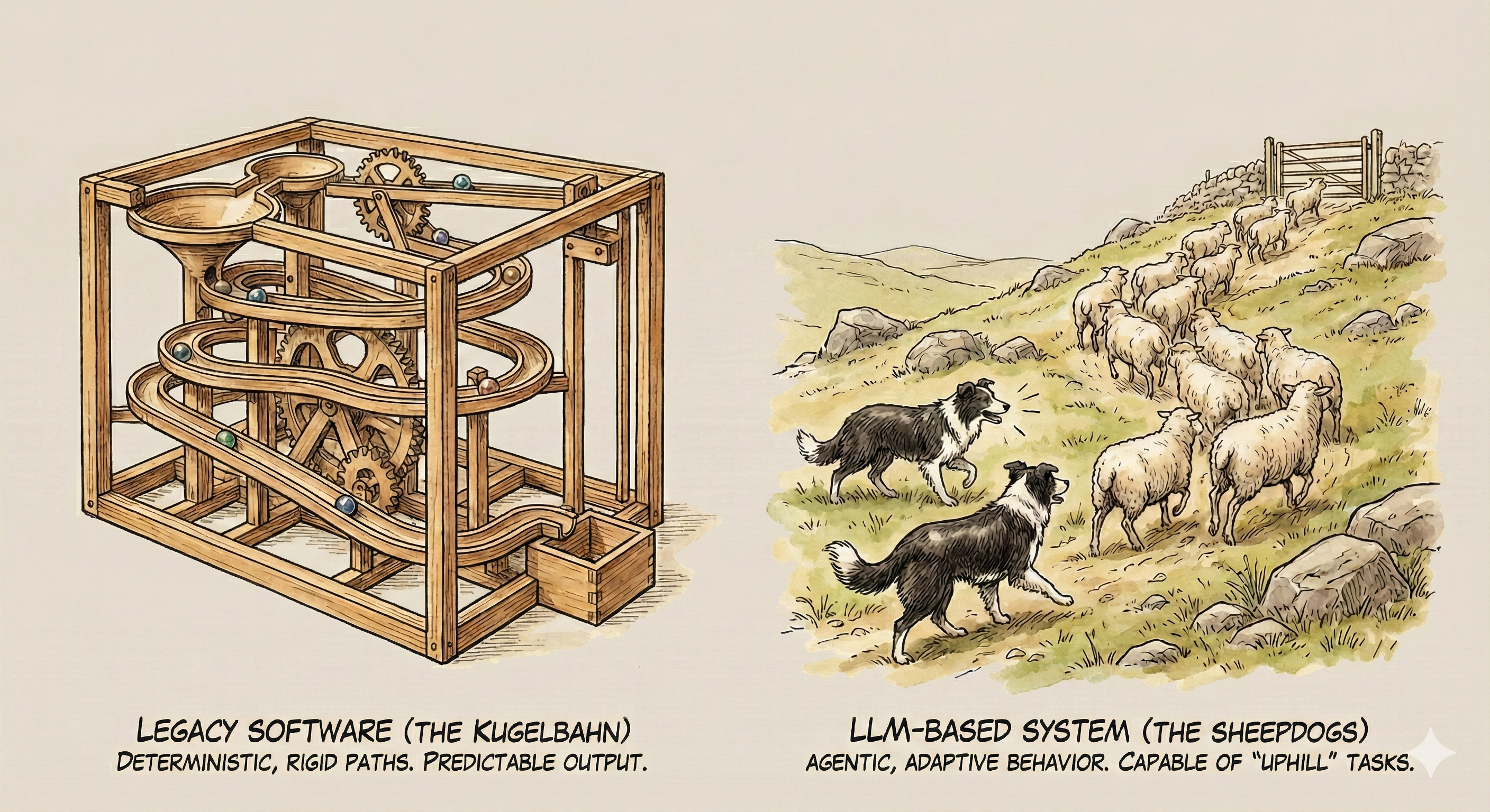
For this particular type of question, I came up with a small analogy to compare LLM-based software vs. legacy software. Legacy software behaves like “Kugelbahn” (German word for Marble roll, or rolling ball sculpture). It works like a well-tuned machine, often performing an amazingly complex job. If something goes wrong, that tends to go wrong at a localized part (say, a rail has been bent), and once you “fix” that part - it tends to work steadily. However, LLM-based software, by contrast, is more like a pair of sheepdogs performing tasks together. They are MUCH more powerful, and can perform things that mere balls cannot perform – such as going uphill, instead of just going downwards, and it even has agency and decides by itself on new situations, and so on. But just like real-world dogs, if things go haywire, the failures are generally far more creative – and do crazy stuff that we might have not predicted. When they misbehave, instead of “fixing”, you put leashes, or set bounds with guardrails, to guide them and to keep them under control.

I find this analogy working well for my colleagues, especially as it naturally leads us into concepts like putting leashes and guardrails, which is a different “mode” of interacting with software to improve the results. However, this opens a more technical question that is tricky (means, needs longer space) to answer. The analogy is actually leading us into “so there is something fundamentally different to LLMs, that it is more lively, and inherently random and unpredictable”. This is a hard question to answer accurately briefly. Because the answer is ‘No, but also Yes’ – and understanding why requires digging into how LLMs actually work.

It is an interesting topic, and may help us understand better how LLM-based software works with us. So I decided to write a two part article about this. In this post, I will first explore technical source of randomness in LLM processing – what is the source of randomness in LLM-processing? Namely, running “the same input” 100 times, can we always get the same result? If not, why not? And in the part 2, I will visit bigger and broader issues around LLMs: that you cannot easily reason about how two “different similar inputs” would behave. Your customer support LLM pipeline might work perfectly 99 times on passing opening hours of a ski shop, then mysteriously suggest that you cannot trust the written opening time, and the customers should always try to call the shop to make sure, on the 100th. Why does it do so? And how can we mitigate that?

Randomness and Neural Network

Neural networks, including LLMs, run on “normal” computer hardware: they might run on exotic pieces such as GPUs, TPUs, NPUs or whatever chips marketed for running NNs quickly. But all those systems are still normal computational hardware, and all calculations are fundamentally deterministic. Unless you bring in something like quantum computing, fundamentally all calculations are deterministic: if the same input goes in, always the same output is guaranteed. No magic, no dice rolls - just math.

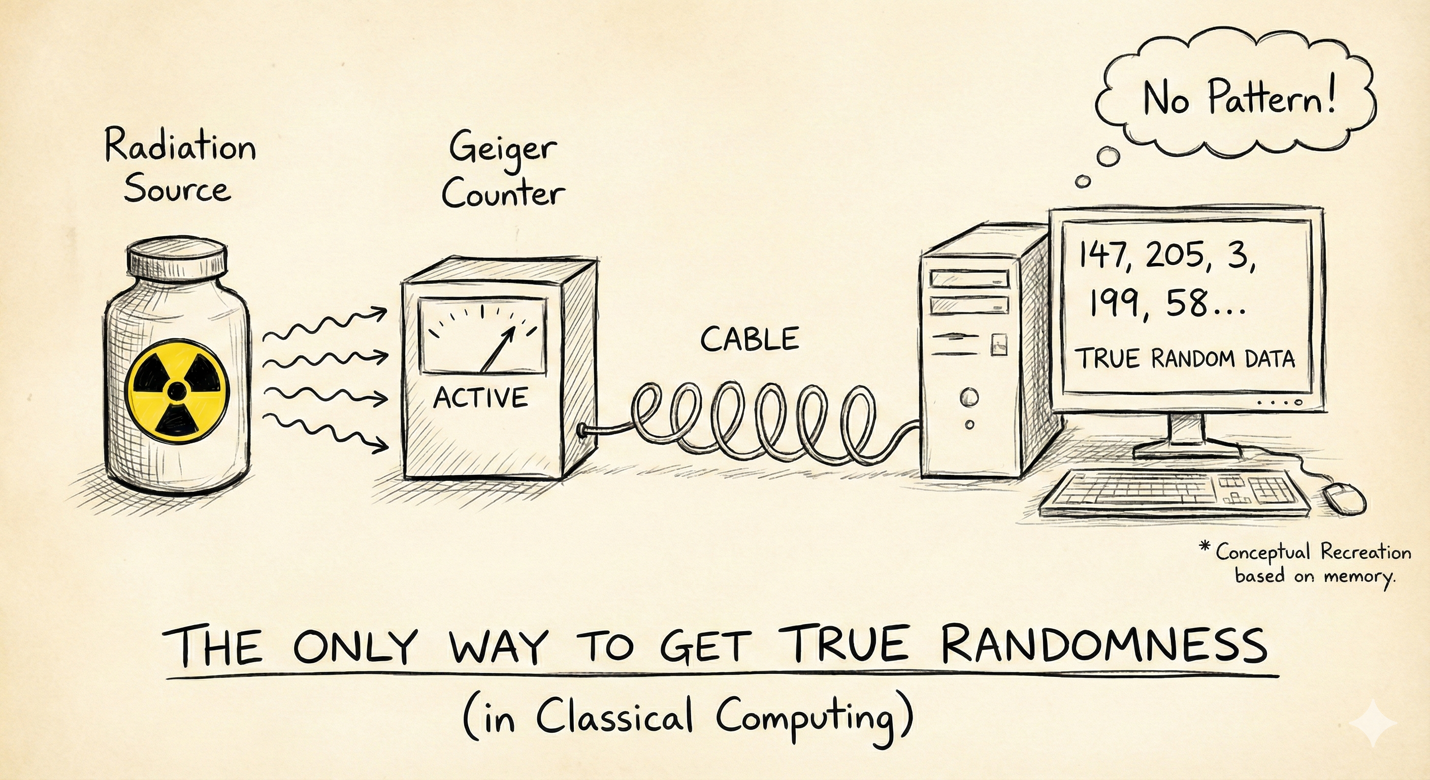
Actually, computers are really bad at providing anything random. I vividly remember a picture that shocked me back in my college days. The chapter started with a drawing of a geiger counter connected to a computer, and introduced this as “the only way to get real randomness”. This easily shocked me and made me shoot back “hey, then what are these rand() call results?”. The textbook naturally knew we would ask this question, and kindly introduced the good old reliable way of “pseudo randomness”. Just as we’ve done since the 19th century, we just read from a book of pre-filled numbers. We get a seed (e.g. a page number), visit that page (open this big book), and read the number out aloud. Same seed, always the same output. This was the textbook’s way of forcing the simple fact to us the students: “there is no randomness in computing”. ¹

We need randomness in many real-life situations. For every such place - our computer programs use pseudo-randomness to make it work. Even in machine learning, we use pseudo-randomness everywhere. When training a neural network, we put initial weights of neurons to slightly different near-zero values (otherwise back propagation won’t even work), we randomly drop out some neurons in the training (so the network doesn’t over-rely on some specific ones and becomes more robust), and we shuffle the training data randomly (so training data will be presented to the model in different orders for each epoch, making it more robust), and so on. All these are seeded, and moreover, “reproducible”.

Sampling of LLMs – How LLMs use (Pseudo-)Randomness

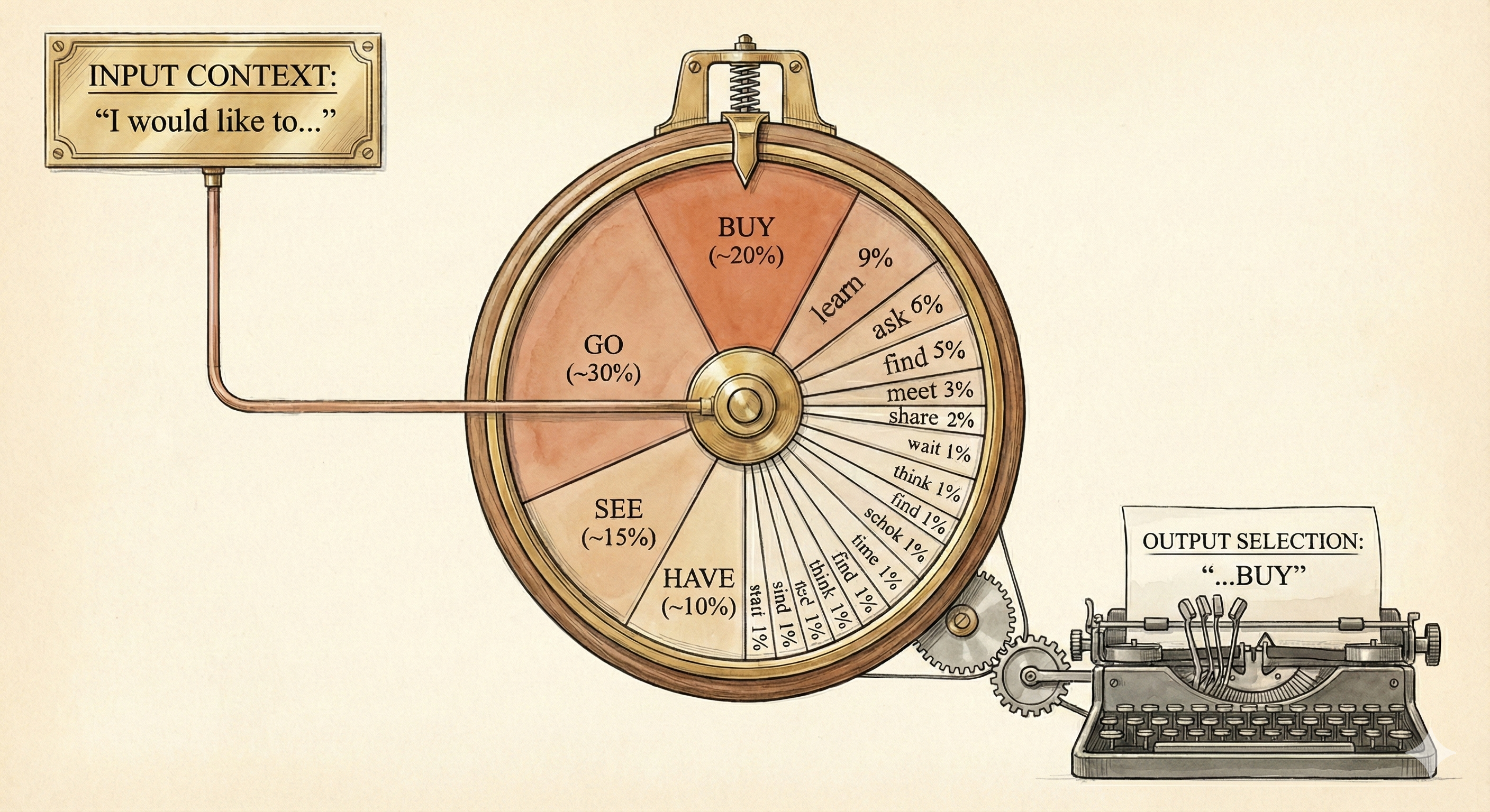
So, how does an LLM actually generate text? LLMs work by predicting the next word, or more precisely, the next “token”. At each step, the model outputs a probability distribution over all possible next tokens. For example, given the prompt ‘I would like to’, the model might assign high probabilities to ‘go’ (30%) and ‘buy’ (20%), moderate probability to ‘see’ (15%), and tiny probabilities to thousands of other tokens. Then, one token gets selected from this distribution. Higher probability tokens are more likely to be picked, but not guaranteed - just like spinning a weighted wheel where some segments are wider than others. This process is aptly called “sampling”.

We can easily see this sampling in action. Let’s say we ask an LLM, “Continue sentence: I would like to”, multiple times. You will get results like this:

• I would like to spend more time exploring …
• I would like to see more kindness and …
• I would like to have a relaxing weekend …
• I would like to buy a new laptop with …
• …

Each time, the sampling process picks slightly different paths. Each path is valid, each weighted by the model’s learned probabilities. This is what gives LLMs their “creative” feel. The same prompt can lead to genuinely different outputs. The sampling makes the generated sentences much more natural, just as we humans would say – when there is enough content to say, human utterances rarely overlap word-for-word, even when the intention is exactly the same. In a similar manner, the sampling process does land on that ‘long tail’ of tiny probabilities shown in the illustration, leading to different word choices.

So we have this sampling process that introduces variation. But what if we want less variation? Or more? LLM APIs typically expose parameters to control this. One common parameter is “top-P”. Instead of considering all possible tokens, top-P says: “only sample from the smallest set of tokens whose combined probability exceeds P%.” So top-P=0.75 means: find the most likely tokens that together make up 75% of the probability mass in the given context - then sample from the reduced set. This cuts off the long tail of unlikely tokens (e.g., fewer surprises).

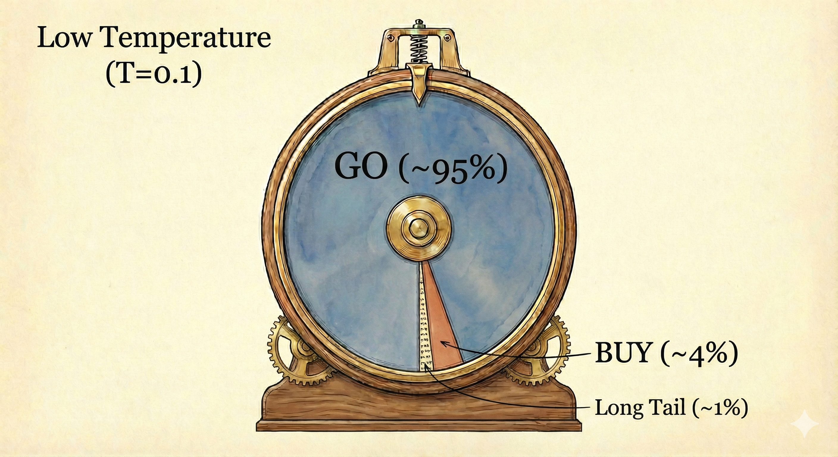
Another common parameter is “temperature”. Think of temperature as controlling how “sharp” or “flat” the probability distribution is. At temperature=1.0, the model uses its original probabilities as-is. Lower the temperature toward 0, and the distribution becomes sharper; high-probability tokens become even more dominant, low-probability ones become negligible. The picture below shows how the original “sampling wheel” changes when we set the temperature to 0.1.

When the temperature is set to 0, sampling effectively disappears: the model always picks the single highest-probability token. This is sometimes called “greedy decoding”. At exactly 0, there’s technically no randomness left - it’s purely deterministic selection. Parameters like temperature and top-p give us some dials – from “creative and varied” (high temperature, high top-P) to “predictable and consistent” (low temperature, low top-P).

But here’s the surprise: even with temperature=0, production LLM models generally don’t give reproducible results. Here are some actual call results from gpt-4.1 with temp=0.0.

Input: Continue the sentence. The sentence: The weather was...

Six consecutive Outputs:

The weather was unexpectedly warm for this time of year, with a gentle breeze carrying the scent of blooming flowers
The weather was unexpectedly warm for early spring, with golden sunlight streaming through the clouds and a gentle breeze carrying the scent of blooming flowers.
...unusually warm for early spring, with sunlight streaming through the windows and a gentle breeze rustling the curtains.
The weather was unusually warm for early spring, with a gentle breeze carrying the scent of blooming flowers through the air.
The weather was unusually warm for early spring, with a gentle breeze carrying the scent of blooming flowers through the air.
The weather was unusually warm for early spring, with golden sunlight streaming through the windows and a gentle breeze rustling the new leaves outside.

So what’s going on here? Why does temp=0 still give us different outputs?

The Hidden Culprit: Batch Processing in Production

The answer lies in how modern production LLM systems actually run — and specifically, in sparse architectures that have become increasingly common in recent years. The most prominent example is Sparse Mixture of Experts (MoE), which is utilized by models like GPTs, DeepSeek, Grok and more, and the architectural approach has become a standard way to scale efficiently. The key idea is simple: not all of the model is used for every request. Instead, the model contains multiple “expert” sub-networks, and depending on your input, different experts get activated. Here’s the catch: which experts activate depends not just on your input, but also on what else is being processed at the same time.

Think of it like this: imagine a committee of specialists answering your question, but they’re simultaneously answering 50 other questions from different people. Your question about weather arrives in batch #4791 alongside queries about cooking recipes, tax law, and Python debugging: and is then handled by, say, expert #800 (literature analysis) and expert #500 (natural science). Run your exact same question again. It then lands in batch #4792 with astronomy questions, poetry analysis, and medical queries, and is then assigned to expert #400 (linguistic) and expert #300 (social science). Different “main writer” for your answer. The assigned experts are deemed capable enough to answer your question, but they are subtly different. The output you get is shaped not just by your prompt, but by this invisible computational context it lands in. ²

Let’s revisit the weather examples from GPT-4.1 with temp=0. They are from different sub-parts of the bigger model, caused by different batch contexts, different expert activations, different numerical paths through the same network. Here’s the practical implication: production LLM APIs handle thousands of requests per second. Your request arrives, gets bundled with whoever else is querying at that millisecond, and processed. You have no control over batch composition. The computational context is invisible to you but affecting the result.

Reproducibility vs. Efficiency

Now, you might be thinking: “Can’t we just fix this?” And actually, yes — some providers now offer “reproducible” or “deterministic” modes, often with a “seed” parameter. In controlled settings like evaluation benchmarks, this works beautifully: same seed, same input, same output. Perfect for running the same evaluation suite multiple times and getting consistent scores.

But here’s the catch: truly reproducible modes often require fixed batch sizes (sometimes batch=1, processing one request at a time) or dedicated compute instances. This can reduce throughput by 10-100x depending on the system. Suddenly your API calls are slower and/or cost significantly more. So in practice, production systems run with dynamic or continuous batching: faster, cheaper, and accepting non-determinism at the single-inference level.

This is why we see non-deterministic LLM outputs from production endpoints - not just from some providers, but from virtually all of them. Unless you run a local instance with single-batch processing, or pay premium costs for dedicated compute, this is simply how production LLMs work. The computational context your request lands in shapes the output you receive, and you have no control over it. This is the reality we live in.

Conclusion

So let’s return to our original question: “Does an LLM have fundamental randomness in it?” The answer, as I said at the beginning, is “No, but also Yes.”

No: There’s nothing inherently more random in LLMs than in other programs. Everything is deterministic in principle. Sampling uses pseudo-randomness (our old friend, the book of random numbers). Batch effects are just computational artifacts—different paths through the same deterministic system.

But Yes: In practice, production LLM systems can’t run deterministically, even with identical inputs and temp=0. Batch composition introduces variance you can’t control: which experts activate (in MoE architectures), what numerical path the computation takes, what other requests share your batch. Methods exist to reduce this (fixed batches, seed parameters, dedicated instances), but we generally live with inference-level non-determinism in production because the alternative is too expensive and too slow.

… and the Bigger Source of Unpredictability

However, there is more to visit on “LLMs seem to be unpredictable”. The bigger contribution comes from something else: you cannot easily reason about how two different but seemingly similar inputs will behave. This is what frustrates users and engineers in production. This is more than sampling variance, or MoE routing. This is emergent behavior from a complex system encountering edge cases in its learned generalizations. The model is trying to solve an inherently underspecified problem – real-world inputs are always ambiguous in subtle ways – and it does so by generalizing from the data it has observed before (training data). Sometimes that generalization is robust. Sometimes it’s brittle. And predicting which is which? That’s the hard part.

Understanding this bigger source of unpredictability – how LLMs generalize, where they fail, and what we can do about it – is the goal of the next article (Part 2).

---

1. Classical computing only, e.g. non-quantum computing. ↩

2. Not all LLMs use sparse architecture, but batch effects still exist even in dense models. The effect is much smaller - typically you might see one word differ after 100 identical tokens, rather than the variation we see in sparse models. But the principle is the same: “different computational context” - batch size affects the order and grouping of floating-point operations, introducing tiny numerical variations that cascade through the network. ↩